John Barrios · Yale School of Management Claude Code for Accounting Research

Module 2: The Empirical Loop on SEC FSDS

Module 2 slides (PDF) · Lab

Module 1 gave you the mental model: files persist and context doesn’t, delegate and then verify, and say what you mean in four parts — file, operation, aggregation, output. That model is correct, and it is also, so far, untested against a real research question. This module is where it gets tested. One accounting question — how has R&D intensity evolved across industries? — travels the entire distance from a vague idea to a verified, publication-style figure, and you watch it happen, then do it yourself with a different measure. The lecture in this module is short and almost entirely mechanical: what the dataset looks like, what the loop’s stages are, and what habits keep the whole thing reproducible. The teaching happens in the demo and the lab, which are the same pipeline run at two different speeds.

The dataset for this module, and the reason it’s the right one to learn on, is the SEC’s Financial Statement Data Sets (FSDS): free, quarterly, credential-free bulk extracts of every XBRL-tagged financial value from every electronic filing the SEC receives. No WRDS account, no Duo push, no institutional subscription — just a zip file you can download to a laptop on a coffee-shop connection. It is also, not coincidentally, structured the way Compustat is structured: a filing-metadata table, a tagged-values table, and a key that joins them. Everything you learn about FSDS in this module previews the shape of the Compustat pipeline you’ll build in Module 4, once WRDS access is live.

NoteLearning objectives

By the end of this module, you should be able to describe the FSDS file structure — sub.txt and num.txt, pipe-delimited, joined on adsh — and explain how it maps onto the shape of Compustat; write and read a six-part opening prompt that specifies the data, the join, the measure, the aggregation, the output, and the paper trail, before any code gets written; run the full empirical loop yourself, end to end, in a single lab session, from an empty folder to a verified figure and a README a stranger could rerun; treat a wrong first-draft figure as the expected first output of a pipeline, not a sign that something is broken, and apply one to three small, targeted refinement rounds instead of one long, over-specified prompt; and apply at least two sanity checks — one benchmark comparison, one plausibility check — before you sign off on any computed result.

The full loop, once, end to end

This module’s design idea is simple: teach the empirical loop by running it, not by describing it. The loop has five stages, and every one of them produces a file, not a conversation. You start from an empty folder. A download script pulls the raw FSDS extracts. A cleaning-and-join script turns the two raw files into an analysis-ready panel, printing its own attrition as it goes. A figure script turns the panel into a labeled, publication-style plot. And a README, written last, states what a stranger would need to type to get from the empty folder back to that same figure. Nothing here is optional, and nothing here happens by talking about it in the chat window; each stage is a named script sitting on disk when you’re done.

The empirical loop: empty folder, download script, clean panel, figure, README — each an artifact on disk, not a conversation.

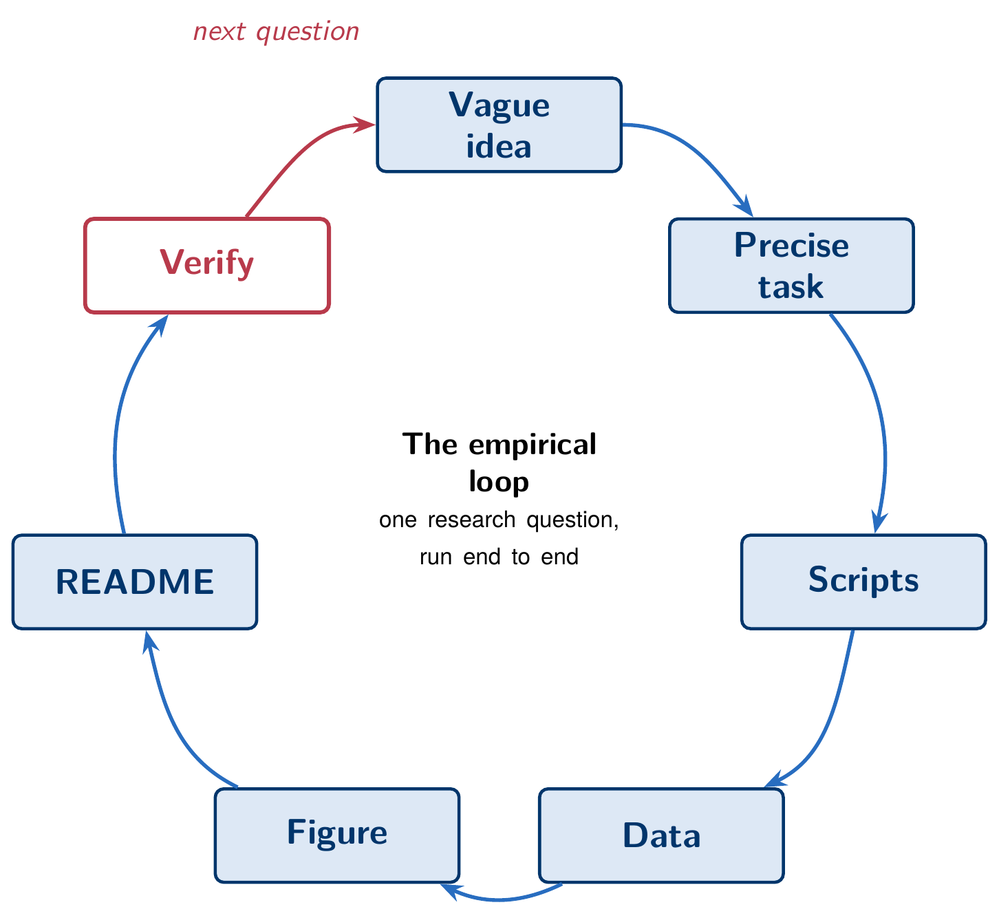
Notice what’s different about this module’s version of Module 1’s habits. Module 1 asked you to write one named script and check one number. This module asks for a full chain of them, each one feeding the next, with the sample size and the reasoning at every step written down as it happens rather than reconstructed afterward. The scale is bigger, but the discipline is identical: state what you want in four parts, write it to a file, verify before you trust it. This module just runs that discipline across a whole pipeline instead of a single step.

SEC FSDS anatomy: two files and one key

FSDS ships as a quarterly zip — one per fiscal quarter, going back to 2009 — and inside each zip are several pipe-delimited text files. Two of them matter for essentially everything you’ll do across this course. sub.txt is the submissions file: one row per filing, giving you the accession number (adsh), the filer’s central index key (cik), its SIC industry code, the form type (10-K, 10-Q, and so on), the fiscal year end, and the period the filing covers. num.txt is the numeric-values file: one row per tagged financial fact inside a filing, giving you the accession number again, the XBRL tag (a controlled vocabulary name like Assets or ResearchAndDevelopmentExpense), the date the value applies to, the number of quarters the value spans (qtrs — zero for a balance-sheet snapshot, four for a full fiscal year of a flow variable), and the value itself.

The join key that ties these two files together is adsh — the filing’s accession number — and it is the single most important fact about FSDS you’ll use across this course. sub.txt tells you who filed what, when, in what industry; num.txt tells you what numbers that filing reported; and adsh is the only reliable bridge between the two. Every pipeline you build in this module starts by reading both files and joining them on that column, and every pipeline should report the row count in each file before the join and the row count after, because a join that silently drops or duplicates rows is one of the most common — and easiest to miss — failure points in any panel-construction pipeline.

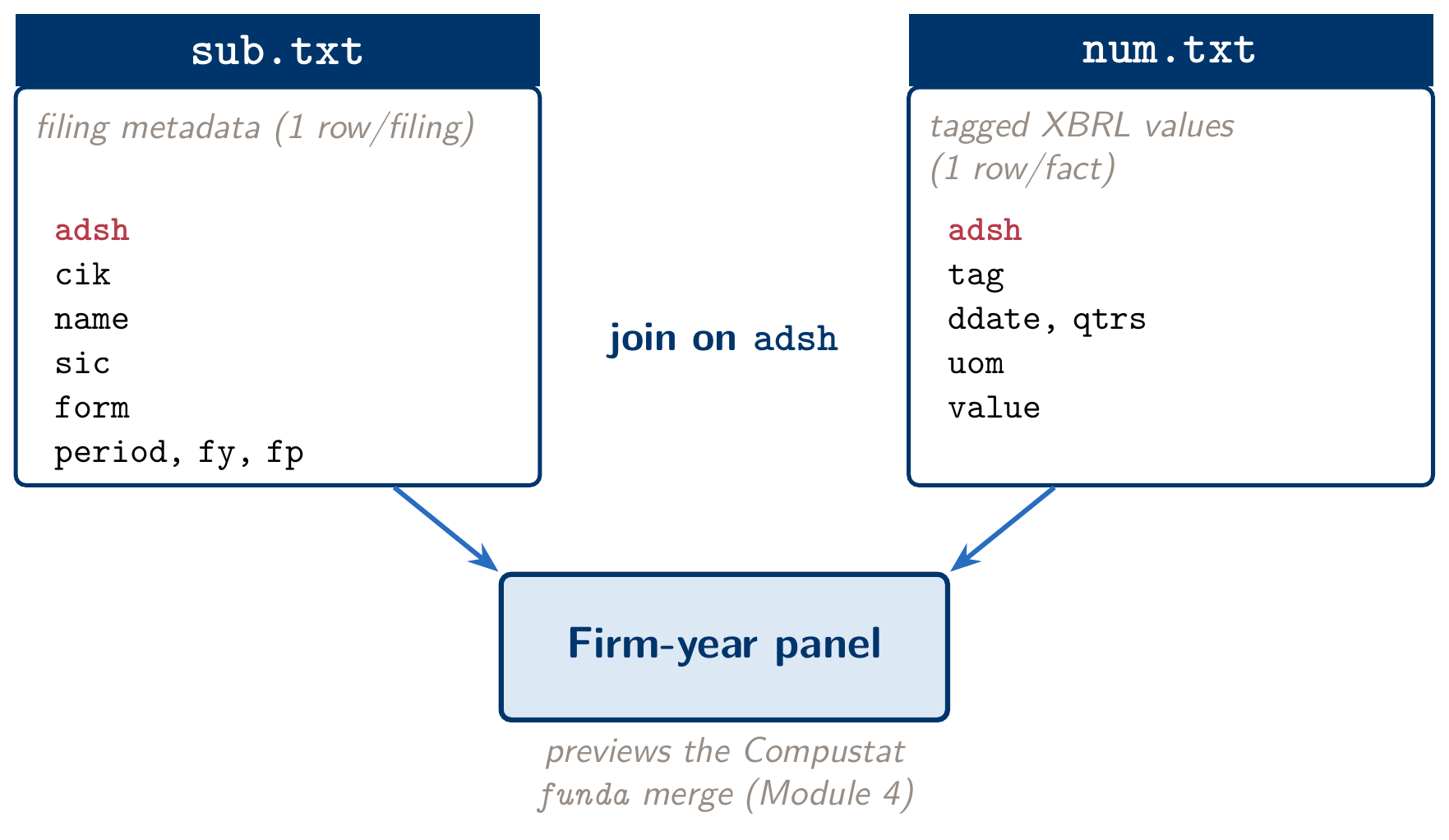
sub.txt and num.txt, joined on adsh: filing metadata meets tagged values.

This structure is also why FSDS is worth learning before Compustat rather than instead of it. Compustat’s funda table is, at a conceptual level, doing the same job num.txt does — one row per firm-year per reported variable — while its company file plays the same role sub.txt plays, giving you the industry code and the identifying metadata you join everything else against. Learn the join-key discipline here, on free data with no account to wait for, and Module 4’s WRDS pipeline will feel like a bigger, better-documented version of something you already know rather than something entirely new.

From vague idea to precise task, one more time

“How has R&D intensity evolved across industries?” is a perfectly good research question and a completely unusable prompt. It doesn’t say which years, which industry grouping, which measure of R&D, which measure of scale, or what the output should look like — and an agent handed that sentence has to guess at every one of those choices, which means you’ll spend your first several turns discovering, one at a time, which guesses it got wrong. Module 1’s four-component habit — file, operation, aggregation, output — is the tool for closing that gap, and this module is where you watch it do real work on a real question rather than a toy one.

Turning the vague version into the precise version means answering, before you type anything: which files (which FSDS quarters, and which two files inside each), which join (on what key, checked how), which measure (R&D expense over total assets — but which XBRL tags, and filtered how), which aggregation (a statistic, by what grouping, over what time unit), and which output (what kind of figure, saved under what name, alongside what underlying table). Every one of those decisions is one a domain expert should be making deliberately, not one an agent should be inferring. The opening-prompt template below is exactly this decomposition, applied in full to this module’s demo question, and it is the single artifact from this module most worth keeping.

Reproducibility as code, not chat lore

Before the opening prompt gets written, three small habits need to be in place, because retrofitting them after the fact is far more expensive than building them in from the start.

The first is empty-folder discipline, and it’s exactly as simple as it sounds: every new project starts in a fresh, empty directory — mkdir ~/lab2 && cd ~/lab2 && claude — so that the first thing the agent sees when it looks around is nothing but this project. This matters more than it looks like it should. An agent that opens into a folder full of last month’s Stata do-files, or a different course’s half-finished scripts, will sometimes let those files leak into its sense of what this project is about; an empty folder rules that out entirely.

The second is named-script discipline, which you met in Module 1 in miniature and which this module leans on hard. Every stage of the loop — download, clean, join, measure, figure — should exist as a named file (download_fsds.py, clean_join.py, build_measure.py, make_figure.py, or whatever names you choose) rather than as a number or a plot that only ever existed inside a chat reply. The test is simple: if you deleted the entire conversation right now, would the pipeline still run? A named script survives that test. An answer typed into a chat window does not.

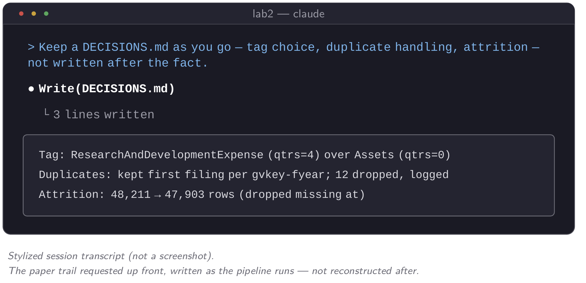
The third is the one that is new in this module: paper-trail prompting. Rather than asking for the analysis and adding documentation afterward as an afterthought, you request the documentation in the same prompt that starts the work — a DECISIONS.md file that records every methodological choice as it gets made (which tag was used when more than one was available, how a duplicate row was handled, why a filter was applied), a LOG.md file with a timestamped line at every major step, and an attrition row — sample size before, sample size after, and the reason for the change — printed every single time the sample shrinks or grows. Asking for this upfront rather than retrofitting it afterward is the whole point: a paper trail requested after the fact is a paper trail reconstructed from memory, and reconstructed memory is the state Module 1 warned you not to rely on.

A paper trail in practice: DECISIONS.md, LOG.md, and an attrition row, each requested in the same prompt that starts the work.

The opening-prompt template

Here is this module’s demo prompt, read slowly and in full — it is the single most reusable artifact of the module, worth keeping verbatim as a template for any empirical question you carry through this pipeline in the future. It has six parts, and the first four are a direct extension of Module 1’s four components; the last two — the join and the paper trail — are what change once a single script becomes a full, multi-stage pipeline.

DATA: Download the FSDS quarterly zip files for these fourteen quarters — Q4 of each year from 2010 through 2023 — from the SEC’s Financial Statement Data Sets page. From each quarter we need two files: sub.txt (filing metadata: adsh, cik, sic, form, fiscal year end, period) and num.txt (tagged numeric values: adsh, tag, ddate, qtrs, value).

JOIN: Merge sub.txt and num.txt on adsh — the filing’s accession number, the only key that reliably links the two files. State the row count in each file before the join and the row count after, and flag any adsh values in num.txt with no match in sub.txt.

MEASURE: R&D intensity, defined as R&D expense divided by total assets for each filer-period. Use the XBRL tag ResearchAndDevelopmentExpense for the numerator and Assets for the denominator. Keep qtrs = 0 rows for Assets (a balance-sheet snapshot) and qtrs = 4 rows for the R&D tag (a full fiscal year of a flow variable). Restrict to form = 10-K.

AGGREGATION: Compute the median R&D-intensity ratio by two-digit SIC code (sic2, the first two digits of sub.txt’s sic column) and calendar year, across all fourteen quarters.

OUTPUT: One line figure, one line per SIC2 industry, R&D intensity on the y-axis and year on the x-axis, formatted for a working-paper draft — white background, labeled axes, a legend, no default plotting-library styling — saved as rd_intensity.png. Save the underlying aggregated table as rd_intensity_by_sic2_year.csv.

PAPER TRAIL: Write every stage as a named script — no output that exists only as a chat reply. Keep a DECISIONS.md recording every methodological choice as it’s made — which tag was chosen when more than one was available, how duplicate rows were handled, any filter applied and why. Keep a LOG.md with a timestamped line for every major step. Print an attrition row — n before, n after, reason — every time the sample size changes.

Read that prompt again and notice what it rules out. There is no ambiguity about which quarters, which tags, which filter, which statistic, or which filename — and there is no possibility that the pipeline ends up living only inside a transcript, because the prompt itself demands scripts and a paper trail as part of the deliverable, not as an afterthought. This is the six-component habit in full, and it’s worth learning well enough that you can produce a version of it for any measure you construct for the rest of this course.

Iteration is not failure

Here is the part that surprises almost everyone the first time they see it: the first-draft figure is essentially never the figure you actually want, and this is completely normal, not a sign that anything has gone wrong. A first pass at the R&D-intensity plot might have the wrong axis labels, an unreadable number of industry lines crowded onto one plot, or an industry grouping too coarse or too fine to show the pattern you’re actually looking for. The fix is not to write one enormous, over-specified prompt that anticipates every possible problem in advance. The fix is small, targeted refinement rounds — fix the axis and labels, look at the result, then adjust the industry-bucket granularity, look again — two or three rounds, each one addressing one specific thing you can see is wrong in the previous draft. Count the rounds as you go; if you’re past three and still not converging, that’s the signal to stop iterating and rethink the request itself, not to keep tweaking indefinitely.

The other kind of iteration in this module is autonomous error recovery, and it’s worth watching closely rather than jumping in to fix yourself. SEC’s servers reject bulk-file requests that don’t identify the requester — a bare “403 Forbidden” the first time a download script runs without a proper User-Agent header. A capable agent reads that error, recognizes what it means, adds an identifying header, and retries successfully, without you typing a single word of the fix.

Autonomous error recovery in practice: a 403 Forbidden, diagnosed and fixed by the agent without you typing a word.

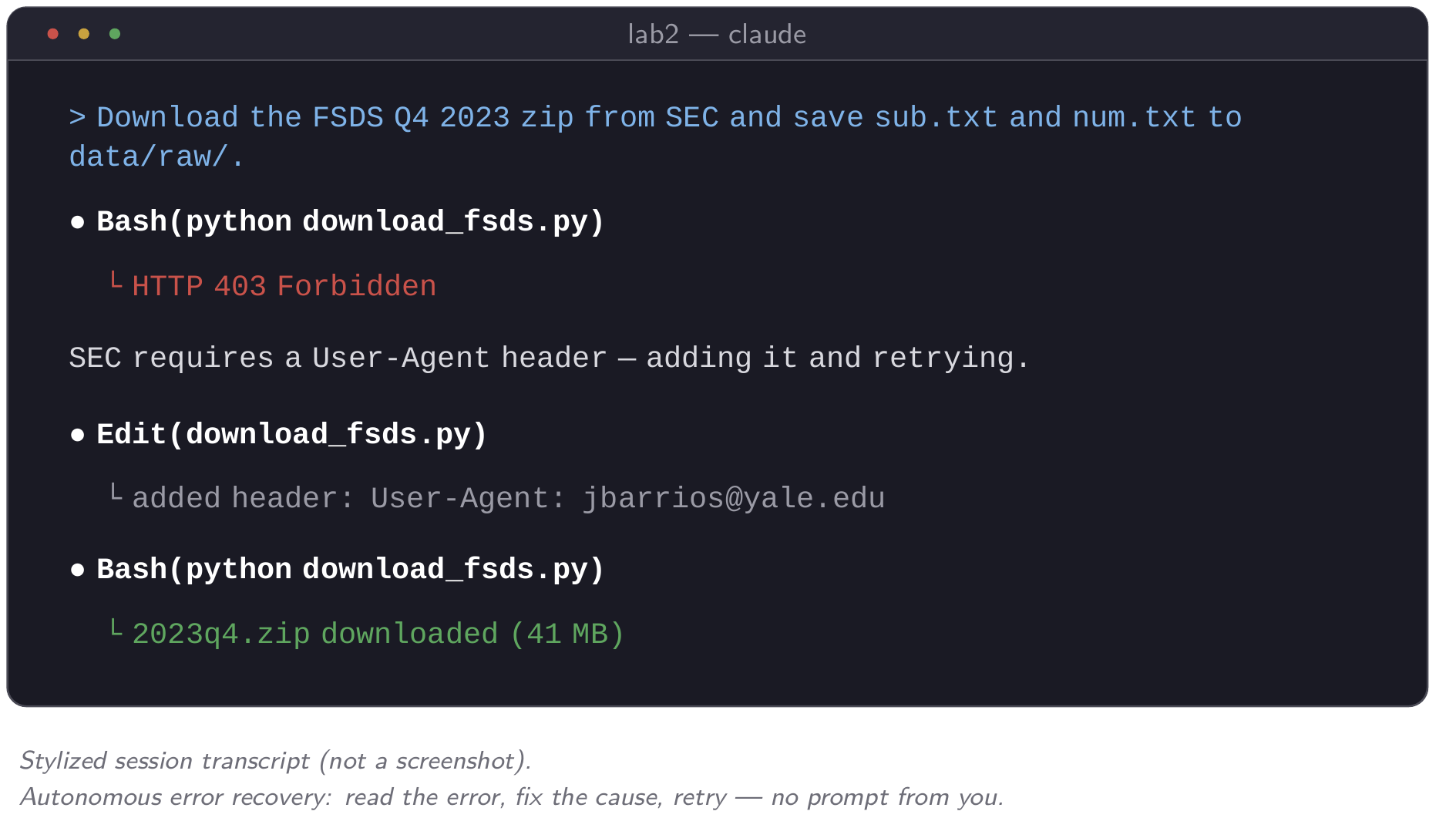
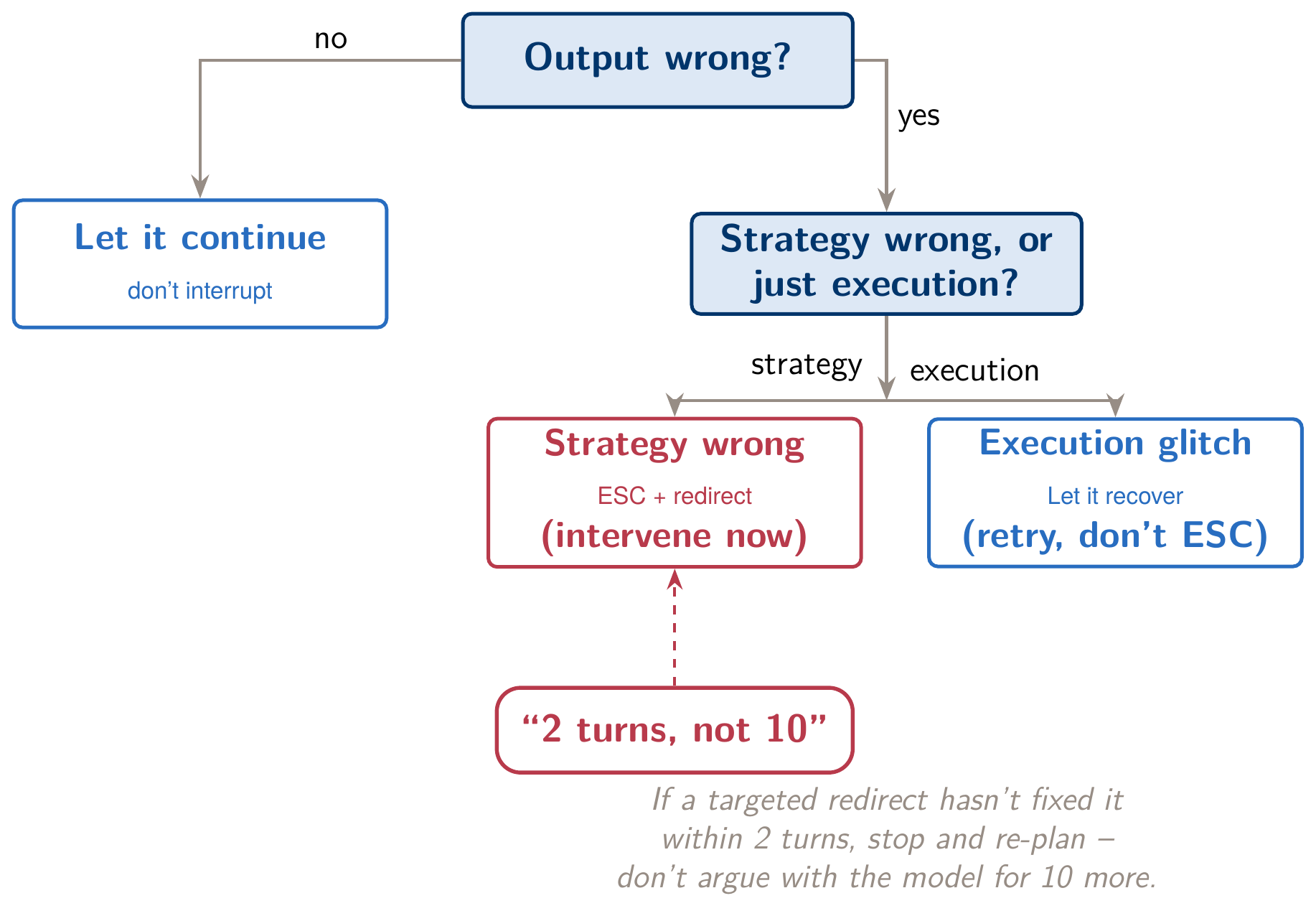
This is a real instance of the same principle Module 1 introduced with redirect-don’t-argue: you watch, you don’t drive, and you only step in when the strategy looks wrong, not every time an intermediate step throws an error. If the agent starts guessing wildly, retrying the same broken approach indefinitely, or heading toward a genuine dead end, that’s the moment to intervene — press Esc, restate the goal plainly, and let it resume from a clean point, exactly as Module 1’s stuck-loop protocol described.

When a pipeline stalls: watch autonomous recovery first, and know the branch point where you step in.

One more thing worth knowing about in this module, briefly, because you may see it happen and wonder what it was: for a long-running search or a task with several independent branches, Claude Code can spin up sub-agents — separate contexts that investigate one piece of a problem and report back a summary, protecting the main conversation’s context budget. This module’s lab is small enough that you may not encounter this at all, and a full treatment of what sub-agents are and how to request parallel ones explicitly is a Module 4 topic. If you do notice one appear in your session, it’s worth a line on your exit ticket; we’ll come back to it.

Sanity checks: two, minimum, before you sign off

Nothing above replaces judgment, and nowhere does that matter more than at the very end, once a figure exists and looks plausible. Before you accept any computed result in this module, run at least two checks, and know what each one is checking for.

The first is a benchmark comparison: pick one or two industries where you already have a strong prior about the answer — pharmaceuticals and software should show meaningfully higher R&D intensity than utilities or retail — and confirm the figure actually shows that. If it doesn’t, something in the tag selection, the filter, or the aggregation is very likely wrong, and it’s much cheaper to catch that now than after the figure has made it into a slide deck. The second is a plausibility check tied to a known event: does the series behave the way you’d expect around a real economic shock? R&D spending patterns around 2020, for instance, should show some visible response to the disruption of that year — not necessarily a specific direction you’ve memorized in advance, but some signature that a real, economically meaningful series would be expected to show. A perfectly smooth, featureless line running through a period you know was turbulent is itself a signal that something upstream has been over-aggregated or mis-constructed.

TipVerify this: name your two checks before you look at the figure

Decide what your benchmark comparison and your plausibility check are going to be before the figure renders, not after. Naming the check in advance keeps you from unconsciously reasoning backward from whatever the figure happens to show to a story that makes it look right. Write both checks down, along with the source you’re checking against, as part of your README — a check that isn’t written down is a check nobody but you will ever know you ran.

These two checks are domain knowledge exercises, not something an agent can substitute for. Claude Code can tell you the median R&D intensity came out at 4% for SIC code 28; it cannot tell you, on its own authority, whether 4% is a plausible number for pharmaceutical R&D intensity in 2019 — that’s accounting and finance judgment, and it is the judgment this course is built to protect.

WarningCommon failure: treating a plausible-looking figure as a verified one

A figure with clean axis labels, a sensible-looking legend, and smooth lines reads as trustworthy — and that visual polish has nothing to do with whether the underlying tag selection, filter, or join was correct. A cosmetically finished figure and a verified figure are different things, and the gap between them is the two checks above. Don’t let a clean plot substitute for actually running them.

The three Module 1 mantras, carried forward

Everything in this module is the same three sentences from Module 1, just doing more work at once.

Files persist; context doesn’t. In this module that means DECISIONS.md, LOG.md, attrition rows, and named scripts at every stage — not just at the end. Trust, but verify — same as an RA. In this module that means two named sanity checks before you sign off on a figure, not a vague sense that it looks fine. Be specific: file, operation, aggregation, output. In this module that habit grows into six parts — data, join, measure, aggregation, output, paper trail — because a full pipeline has more decisions in it than a single script did, and every one of them still needs to be stated rather than inferred.

From here, head to this module’s lab, where you’ll run this same loop yourself on a measure of your own choosing — disjoint from this module’s R&D demo, so your verification is real rather than copied. The lab ends with a hard gate: every student needs a working WRDS tunnel confirmed before Module 4’s flagship lab depends on it, so if you haven’t already tested ssh wrds and a Duo push since Module 1’s homework, do it before you arrive for this module. Two days of runway is the minimum lead time to fix an account or Duo problem through WRDS support — the lab’s closing checkpoint is where that gets confirmed, not scrambled at the last minute.